6월 1주차 그래프 오마카세

Topological Deep Learning: Going Beyond Graph Data

[https://arxiv.org/pdf/2206.00606.pdf]

Why TDA? 라는 질문에 명쾌하게 답을 할 수 있을 논문입니다.

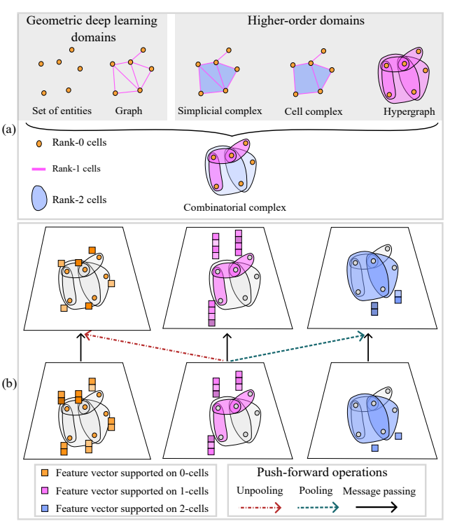
Geometry 문제를 해결할 때만 TDA 를 활용할 수 있다.라는 고정관념을 깬 논문입니다. combinatorial complex neural network 라는 관점을 언급하면서, 기존 Pair-wise , hypergraph 그리고 combinatorial complex (matrix rank) 측면까지 topological 측면으로 잘 설명되어 있습니다. 특히, hypergraph 와 topology 를 결합하여 graph augmentation 도 가능하다는것을 본 논문을 통해 처음 알게되었는데요.

창의력 있고 새로운 인사이트를 논리적으로 잘 설명해놓은 논문이라 생각됩니다. fancy 연구 주제 혹은 ‘rather than hypergraph’라는 니즈가 있으신분들에게 많은 도움이 될 거 같습니다.

실용적인 측면에 관심이 많으신분들은 2.2 The utility of topology 부터 보시는걸 추천합니다.

1.Building hierarchical representations of data.

2.Improving performance through inductive bias.

3.Construction of efficient graph-based message passing over long-range.

4.Improved expressive power.

TDA 를 통해 얻게되는 4가지 이점을 언급하며 머신러닝에서도 유용함을 자세히 설명합니다. 뿐만아니라, graph classification 에서 pooling 이 필수적인 과정인데 이 과정을 topolgy 로 대체하는 부분또한 굉장히 재밌습니다.

GPT-GNN: Generative Pre-Training of Graph Neural Networks

[https://arxiv.org/pdf/2006.15437.pdf]

Introduction

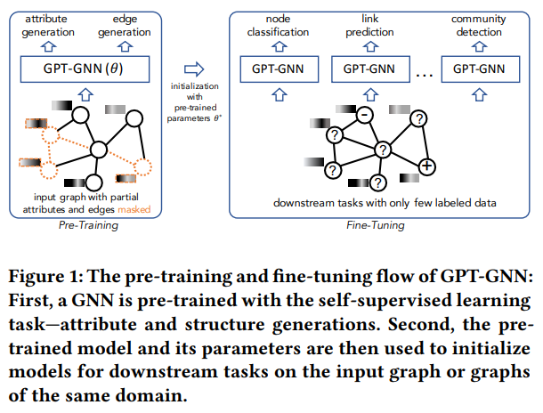
NLP , CV 분야에서는 labeling tool 이 존재할만큼, 굉장히 범용적인 영역인데요. 이와 대조적으로 graph dataset 은 상대적으로 labeled 하기가 어렵습니다. ‘무슨 관계(엣지)’ 인지에 대해 정의(labeling)하기가 까다롭다는게 가장 큰 이유인데요. 논문에서도 이 부분을 언급하며 labeled graph dataset 에 대한 니즈를 pre-training 그리고 Fine-tunning skill 로 접근해보고자 시도합니다. 그렇다면 pre-training 이 핵심일텐데요. 과연 어떻게 data intrinsic distribution 을 보존하면서 weight 를 얻어낼 수 있을까요? 그 방법들에 대해 이야기합니다.

Preliminiary

GNN ‘s pretraining and fine-tunning

Graph neural networks (GNNs) are typically trained using a two-step process: pre-training and fine-tuning. In the pre-training phase, the GNN is trained on a large-scale graph dataset to learn meaningful representations of nodes and edges. The learned representations capture structural and relational information present in the graph.

1. Data preparation: The first step is to prepare the graph dataset for pre-training. This involves representing the graph as a set of nodes and edges, where each node and edge has associated features or attributes.
2. Encoder architecture: The next step is to define the architecture of the graph neural network. GNNs typically consist of multiple layers of graph convolutional operations that aggregate information from neighboring nodes and update the node representations. The exact architecture can vary depending on the specific GNN model being used.
3. Pre-training objective: A pre-training objective is defined to guide the learning process. The objective typically involves reconstructing or predicting some aspect of the graph structure. One common objective is node-level representation learning, where the GNN is trained to predict the attributes or labels of nodes in the graph based on their local neighborhood.
4. Pre-training algorithm: The pre-training algorithm iterates over the graph dataset and updates the parameters of the GNN to minimize the pre-training objective. The algorithm typically uses gradient-based optimization techniques, such as stochastic gradient descent (SGD), to update the network parameters.

Input: Graph dataset G, GNN architecture GNN, Pre-training objective objective, Learning rate lr, Number of epochs N

Initialize GNN with random weights

for epoch in range(N):
    for graph in G:
        for node in graph.nodes:
            neighbors = get_neighbors(node)  # Get the neighbors of the node
            node_features = node.features  # Get the features of the node
            
            # Update the node representation using the GNN architecture
            updated_node_representation = GNN(node_features, neighbors)
            
            # Compute the pre-training objective
            loss = objective(updated_node_representation, node.labels)
            
            # Compute gradients and update weights
            gradients = compute_gradients(loss, GNN.parameters())
            update_weights(GNN.parameters(), gradients, lr)

Summary

label 되어있지 않은 데이터로부터 label 을 적용해주는게 본 논문의 핵심입니다. 그렇다면 label 은 어떻게 정의할까요? 본 논문에서는 label 을 정의하기 위해 attribute 와 structure dependency 를 활용합니다. 이 dependency 는 BERT 에서 많이들 접해보셨을 Masking technique 와 permutation technique를 적용하는데요. 간단히 말씀드려보자면, node 그리고 edge 를 permutation (random order) , mask 했을때 각각의 node attribute , edge (structure) 에 대한 분포를 비교해보는겁니다. 이 과정을 반복함으로써, 어떤 특질이 있고없고 여부에 따라 상관성이 관찰되는데, 그 상관성을 기반으로 label generation을 해주는거죠.

Insight

Summary 에 언급한 부분 이외에도 minor 한 부분으로 1. attribute & edge generation loss design 2. additive embedding queue , large-scale graph subsampling 라는 재밌는 아이디어들이 존재합니다. 그 중 additive embedding 은 generation 시마다 sub-sampling 을 하게 될텐데, 그 sub-sampling 에 Queue 관점을 접목해서 large-graph 에서도 parallel 하게 generation 할 수 있게 만듭니다.

Graph Neural Networks can Recover the Hidden Features Solely from the Graph Structure

[https://arxiv.org/pdf/2301.10956.pdf]

Introduction

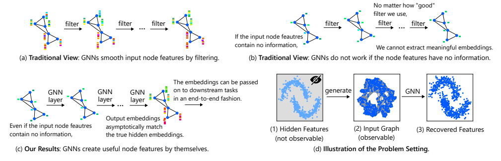
GNN 핵심인 Message passing propagation, aggregation 그리고 update 를 하기 위한 node , edge feature가 핵심인데, 만약 이 feature 라 uninformative 혹은 non-exist 라면 어떨까요? 본 논문에서는 , 그 문제를 완화해보고자 hidden feature(내재되어 있는 특성을 반영) 하기 위한 아이디어를 제안합니다.

Preliminiary

Correct and Smooth technique , the contrastive perceptive in this paper. it was deal with post-pre concept. not including the embedding space.

The Correct and Smooth (C&S) procedure involves two post-processing steps: (i) an "error correlation" step that spreads residual errors in training data to correct errors in test data, and (ii) a "prediction correlation" step that smooths the predictions on the test data. These steps are implemented via simple modifications to standard label propagation techniques from early graph-based semi-supervised learning methods.

The Correct and Smooth (C&S) procedure uses label propagation techniques to capture informative distributions of the graph. The two post-processing steps in C&S are designed to exploit correlation in the label structure of the graph, which helps to improve the accuracy of node classification. However, it's important to note that C&S does not rely on learning over the graph and only uses it in pre-processing and post-processing steps.

Summary

내재되어있는 그래프 특성? 의문점이 드실 부분이라 생각됩니다. 본 논문에서는 그래프 자체 구조를 통해 feature 를 도출하는 방안 (recovery hidden feature) 를 제안합니다. 바로 그래프 구조에서 저희가 찾지 못한 인사이트를 찾아내는거죠. 기존에 저희가 feature 가 없을때 적용하던 degree, spectral view(laplacian) 등 혹은 K-nn graph 과는 다른 관점으로 접근합니다.

바로, new distance 그리고 new expressive solution 을 통해 inductive bias 를 추출하는겁니다. 굉장히 신선한 관점입니다. graph inherent feature 를 찾기위해 그래프 고유성에 조금 더 집중하는거죠. 예를 들면, real-case 에서의 2-hop 이였던 노드들이 과연 embedding space 에서도 2-hop 일까요? 실험 결과 그렇지 않다라는 한계점이 존재하였기에 앞서 언급한 node distance , node expressive 를 적극 활용하여 적절한 real world feature 를 embedding feature 까지 적용할 수 있는 방식을 고안했습니다.

Insight

실험부분에서 ground-truth vs. traditional method vs. our method 삼파전을 관찰할 수 있습니다. performance result 만으로 embedding value 를 간접적으로 가늠했던 제 방식에 대해 통찰을 주는 부분이였습니다. 여러분들도 한 번 보시고 그 임베딩 결과가 performance result 까지 어떻게 이어지는지에 대해 한 번 공부해보시면 좋을거 같습니다.

preliminary 에 적어둔 Correct & Smooth 는 error 기반으로 diffusion 을 발생시켜 distribution capture 을 통해 performance 를 높이는 관점이라면, 본 아이디어는 embedding space 에 치중합니다. 이 두 관점이 상호 배타적으로 보이겠지만, 공통점이 있습니다. 바로 structure 에 치중한다는건데요. 한쪽은 real space에서의 structure 다른 한쪽은 embedding space structure, 이 둘을 결합해보면 어떤 시너지가 날지 궁금하네요. 여러분께서 한 번 시도해보시면 어떨까요?