7월 4주차 그래프 오마카세


Linkedin Graph Database? (industrial session)
소셜 네트워크로 유명한 기업이죠 linkedin, ‘you may know this person’ 이라는 message 가 사용자로 하여금 이목을 끌어, 새로운 관계를 발굴하고 맺어주는 시스템이 핵심 기술이라 할 수 있습니다.
근데, 한번쯤 궁금하지 않으셨나요? 나와 ‘아는사람’ 의 ‘아는사람’ 그리고 ‘아는사람:*..n’ , higher-order relationship 을 실시간으로 어떻게 도출할까? 직관적으로 scan-cost 만 살펴보아도 굉장히 큰 연산량이 필요할거라는 생각이 들텐데요.
그 기술의 핵심에는 바로 ‘Graph Database’가 존재했습니다. linkedin, social network 를 주로 다루는 테크기업에서는 graph 를 어떻게 다루고 있을까요? GDB 를 도입하게 된 배경부터 실활용 예시까지 알아보겠습니다. 이번주 오마카세에서는 주방장이 판단하기에 핵심 Quote 만을 플레이팅 해놓겠지만, 개인적으로 꼭 읽어보셨으면 합니다.
LIquid: The soul of a new graph database, Part 1
[https://engineering.linkedin.com/blog/2020/liquid-the-soul-of-a-new-graph-database-part-1]
Overview
describe how graph data relates to applications, specifically the in-memory graph of structures commonly used as “models” in the sense of “Model-View-Controller” as understood by graphical applications.
Graph data 가 기존 데이터 베이스에서는 어떤 형식으로 저장되고 있었으며, 무슨 문제 때문에 Linkedin에서 하고자하는 (second-order graph recommendation) task 에선 부적합한지에 대한 이야기를 주로 다룹니다.
Query & scan cost , Database engine 그리고 data schema view 3가지 분류를 통해 문제를 나열하고 어떤식으로 접근할지에 대한 추상적인 아이디어에 대해 이야기합니다.
Quote1
LIquid’s query processing engine achieves high performance by using dynamic query planning on wait-free shared-memory index structures.
Quote2
While heavily optimized for both space and speed, these index structures are the basic index data structures that LIquid uses.
LIquid: The soul of a new graph database, Part 2
[https://engineering.linkedin.com/blog/2020/liquid--the-soul-of-a-new-graph-database--part-2]
Overview
how graph data can be stored in a conventional relational database, and why conventional relational databases don’t work very well for this purpose. Rather than scrapping the relational model completely, we will go on to show how relational graph data can be processed efficiently.
Quote1
Concretely, at terabyte scale, an immutable B-tree will probably have at least three levels, with only the first being relatively hot in the L1 cache. A single probe will require two probably-uncached binary searches, easily dozens of L3 cache misses to materialize a single edge. Mutability will make this performance worse. In contrast, the index structures that we describe in “Nanosecond Indexing of Graph Data with Hash Maps and VLists” (presentation) will do a probe for a single edge in either 2 or 3 L3 misses.
Quote2
LIquid uses a cost-based dynamic query evaluator, based on constraint satisfaction applied to a graph of edge-constraints. In this context, “dynamic” means that the query plan is not known when evaluation starts. In a traditional SQL query evaluator, the query plan (a tree of relational algebra operators) is completely determined before evaluation starts. In contrast, LIquid’s evaluator establishes path consistency of the result subgraph by repeatedly satisfying the cheapest remaining constraint.
Graph Database 도입에 대해 고민이신 분들에게 도움이 될 글입니다. 우리가 왜? GDB 를 사용해야하는지에 대한 명확한 목표설정과 그에 대한 근거. 목표 설정 이 후 기존 방법론에서 어떤 문제가 있는지 문제정의 그리고 구체적인 해결방안들이 담겨있습니다.
GDB 회사들의 performance table을 무작정 보는것 보다 위 2부작 포스팅을 읽고 그 performance power 가 어디로부터 나오는지에 대한 배경 지식을 쌓으신 후에 접근하시는게 훨씬 합리적인 의사결정을 할 수 있을거라 장담합니다. 다만, 글을 읽어가다 보이는 Database 관련 용어들이 여러분들의 흐름을 방해할 수 있기에 옆에 chatgpt 선생님을 모시고 함께 읽으시는걸 추천드립니다.
part1, 2를 통해 만들어진 GDB 가 어떻게 활용되고 있는지 궁금하신 분들을 위해 가져온 포스팅입니다. 여러분들의 궁금증이 해소되었으면 하네요.
Graph가 Linkedin 에 구체적으로 어떻게 기여했는지 수치와 함께 적혀있는 포스팅.
How LIquid Connects Everything So Our Members Can Do Anything
Our implementation of LIquid for PYMK has delivered some exceptional outcomes. The QPS has increased from 120QPS to 18000QPS, latencies have dropped from over 1s to under an average of 50ms, and CPU utilization has decreased by more than 3x.
Analytics view , Graph 가 분석가들에게 어떤식으로 도움을 주는지 적혀있는 포스팅.
From the Economic Graph to Economic Insights: Building the Infrastructure for Delivering Labor Market Insights from LinkedIn Data
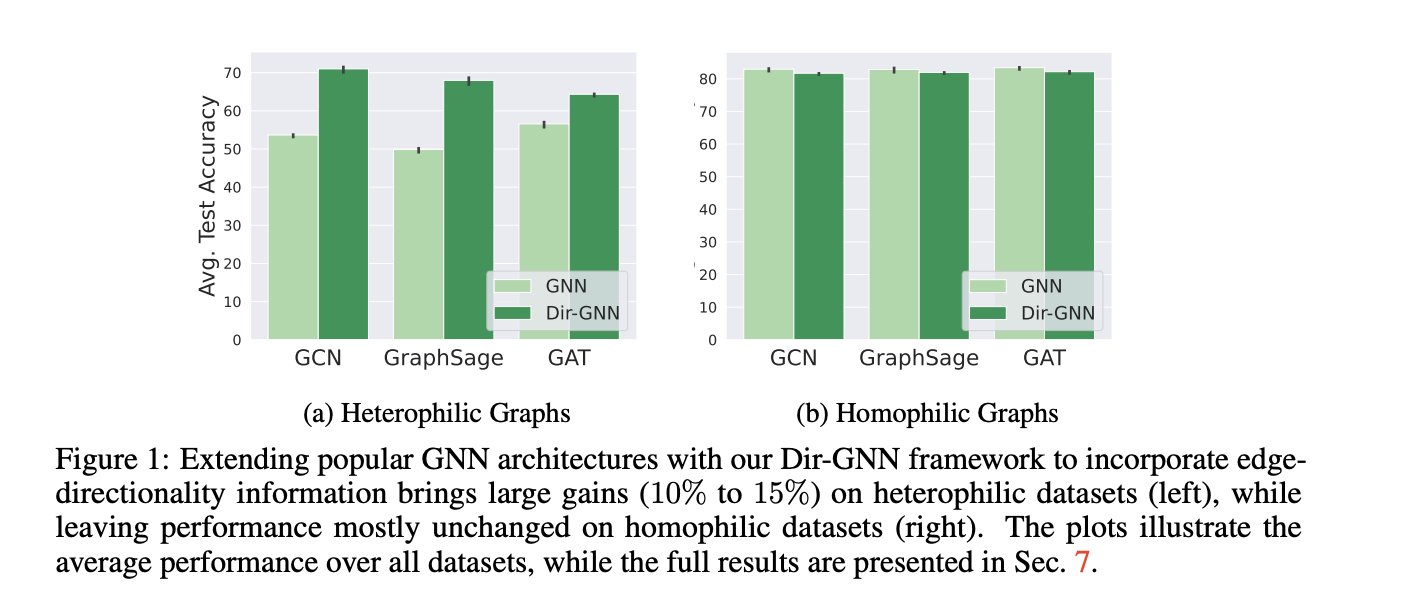
Edge Directionality Improves Learning on Heterophilic Graphs
[https://arxiv.org/pdf/2305.10498.pdf]
Introduction
GNN 에서 간만에 보는 data-centric approach 이지 않을까 싶습니다. GUG 세미나 때 나온 질문이 오버랩되며 논문이 술술 읽혔습니다. 바로, FDS를 위한 그래프 모델링에서 directed 를 고려했는지에 대한 질문이였습니다. 결국, FDS 에서는 방향성을 토대로 거래에 대한 ‘의도’를 표현하는데요. 주고 받음의 의도가 중요한 부분에서 저는 이를 생략했었기에, 연구 설계 측면에서 누락한 부분이 존재했구나 하며 아차 싶었던 순간 이였습니다.
다시 논문으로 돌아와서, 논문에서는 그래프 중요 특성 중 하나인 ‘방향성’ 을 고려하여 message passing 에 접목합니다. ‘forward’ , ‘backward’ 에 따라 node feature 를 각각 반영하여 Reduce 까지 이전 Message passing 과는 ‘방향성을 개별로 반영하여 적용한다’ 라는 점과는 딱히 차이점이 없습니다.
Preliminary
[Homophily and Heterophily]
- Homophily
Homophily refers to the tendency of nodes in a network to be more likely to connect or form relationships with other nodes that have similar attributes or characteristics. In other words, like-minded or similar nodes are more likely to be connected in a network. These attributes can be demographics, interests, beliefs, behaviors, or any other measurable characteristics.
Real-world case example: Social networks often exhibit homophily. People tend to form connections with others who share similar interests, backgrounds, or ideologies. For instance, in an online social network, users interested in photography are more likely to be connected to other photography enthusiasts, forming a cohesive subgroup within the larger network.
- Heterophily
Heterophily, on the other hand, refers to the tendency of nodes in a network to form connections or relationships with nodes that have different attributes or characteristics. In other words, nodes with diverse traits are more likely to be connected in a network.
Real-world case example: Heterophily can be observed in collaboration networks, where individuals with different expertise or skills are more likely to collaborate on projects. For instance, in an academic collaboration network, researchers from different disciplines may come together to work on interdisciplinary projects, leading to a diverse and interconnected research community.
Summary
왜 directed 가 중요한지에 대해서부터 서술하며, homophily & heterophily metric 을 통해 EDA 그리고 directed를 반영한 message passing까지 예상하시는 전개 그대로입니다.
유념하시면 좋을 부분은 expressivity 인데요. 다른 비정형 데이터를 다루다가 graph 로 넘어오시는 분들께서 가장 어려워하시는 부분 중 하나가 바로 ‘추상적이다’ 였습니다. 예를 들면, 이미지 자연어와 같은 경우는 데이터를 명확하게 분별할 수 있는 반면에, 그래프는 A와 B 가 연결되있다 하더라도, 어떤 구조로 연결되어있느냐에 따라 또 의미가 달라지기 때문에 굉장히 애매모호한 부분이 존재한다. 였습니다.
이를 해결하고자 ‘graph expressivity power’가 대두되고 있구요. 이 부분을 결국 기존 topology + @인 directed 추가 여부에 따라 expressivity 가 좋아질것인가 , 오히려 나빠질것인가에 대해 appendix 에서 다뤘습니다.이를 notation 과 Synthetic data experiment 를 통해 결과 그리고 그에 대한 해석을 논리적으로 잘 전개해놓았습니다.
Insight
한계점이 명확해보입니다. 방향성이 존재함에 따라 1. Lapalcain matrix 정방행렬을 도출하기에 한계가 존재하여, spectral approach 적용이 어렵다. (너무 당연하긴 하네요.. spatial 에 특화되어 있긴 하니깐요.) 2. 2hop, 3hop 등 1hop 초과되는 모델인 diffusion , long-range task 에서는 제 힘을 발휘하기가 어렵지 않을까 입니다. 바로 방향성을 고려한 message passing 경우의 수가 기하급수적으로 증가하기 때문인데요. 기존에는 node feature * graph structure 만을 고려했다면 , 방향성을 고려한다면 node feature * graph structure (left) , node feature * graph structure (right)를 hop마다 반영해야하기 때문이죠.
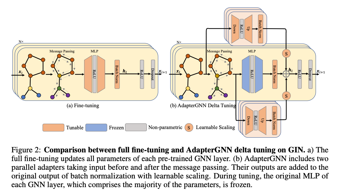
AdapterGNN: Efficient Delta Tuning Improves Generalization Ability in Graph Neural Networks
[https://arxiv.org/pdf/2304.09595.pdf]
Introduction
대용량 데이터 시대에 살고 있다라고 해도 과언이 아닐 만큼 대용량 데이터를 다루는 기술의 중요도가 날이 갈수록 커져가는게 체감되는 요즘입니다. AI 분야에서도 마찬가지인데요. 여러 활용 방안들이 있겠지만 오늘은 그 중 대용량 데이터를 ‘잘’ 학습하여 일반화성능에 기여하고자 하는 기술인 ‘전이 학습’ 에 대해 다뤄보고자 합니다.
말 그대로 ‘전이’ 하는 기술을 나타내며, 대용량 데이터를 학습시키는 과정인 ‘사전 학습’을 통해 도출된 파라미터를 타 task에 적용을 하는거죠. 흔히 ‘fine-tunning’ 이라고도 하며, 목표는 다음과 같습니다. 사전 훈련된 모델에서 배운 지식을 활용하고 이를 새 작업 또는 데이터에 적용하여 새 작업에 대한 모델의 성능을 향상시키는 것입니다.
아름다운 기술이라 불리우는 fine-tunning 모든게 완벽해보이고 굉장히 유용해보이지만, fine-tunning 에는 다음 두 가지 문제가 존재합니다 첫번째는 , 기껏 pre-training 해놓은 parameter 를 희석시켜 forgetting 해버리는 문제입니다. Layer freeze 를 통해 pre-trained paramters 를 활용하더라도 fine-tunning layer에서 paramter 를 잘못 학습한다면 도루묵이 되버리는거죠. 다음 두번째는 바로 large paramter 대비 너무 작은 dataset를 training 해야하는거죠. over-fitting 이 발생할거같다? 라는 불안감이 엄습합니다.
위 두 가지 문제, 1.Parameter forgetting 2. small dataset task 를 delta-tunning 에서는 generalization bounds 를 통해 해결해보려고 시도합니다.
Preliminary
[delta-tunning?]
Here's a hypothetical example of how "delta tuning" might be applied in a database scenario:
Suppose you have a large-scale database system handling user requests. You want to optimize the performance of the database for read-heavy workloads. Instead of making significant configuration changes all at once, you decide to use "delta tuning" to make incremental adjustments and measure their impact.
Step 1: Baseline measurement: You first establish a baseline performance metric for the database under its current configuration. This includes measuring metrics like response time, throughput, and resource utilization.
Step 2: Incremental changes: You identify a configuration parameter that might affect database performance, such as the number of connections allowed or the size of the database cache. You then make a small change to that parameter, such as increasing the cache size by a modest amount.
Step 3: Measurement and comparison: After applying the incremental change, you run performance tests again and compare the results to the baseline. You observe how the change affected performance metrics and whether it led to any improvements.
Step 4: Repeat and iterate: Based on the results of the previous step, you either keep the change, revert it, or try another small incremental change to a different parameter. You repeat this process, making adjustments and measuring performance iteratively until you find the optimal configuration for your specific workload.
The "delta tuning" approach allows you to avoid drastic changes that could potentially lead to adverse effects or disrupt the system's stability. Instead, you make small, controlled modifications and continually assess the impact, gradually converging towards an optimized configuration.
Summary
AdpaterGNN 은 사전 훈련된 모델과 표현력이 뛰어난 어댑터를 활용하여 그래프 신경망(GNN)의 일반화 능력을 향상시키는 동시에 미세 조정해야 하는 매개 변수의 수를 최소화합니다.
핵심 아이디어인 델타 튜닝 접근 방식을 간단하게 설명해보자면, GNN , MLP 각각 사전/사후에 adapter layer 라는 레이어를 추가해서 adapter weight를 보존합니다. 최종적으로 이 weight 들을 기존 레이어와 추가해서 총 3가지 측면으로 학습된 weight를 통해 추론합니다. 이렇게 되면 결국, pre-trained 의 파라미터 그리고 task-agnostic 파라미터를 모두 병렬적으로 반영할 수 있는거죠.
이렇게 구현할 수 있는 기술 뒷면에는 ‘scaling’ , ‘Transfer Gain Boundary’ 라는 기술이 존재합니다. Scaling 은 레이어들로부터 각기 다른 파라미터들이 도출될텐데, 이를 모두 통일하기 위한 기술 그리고 Transfer Gain 은 어떤 파라미터가 중요한것인가에 대한 기준을 Parameter by Error 를 통해 도출하여 최적의 boundary 를 뽑아냅니다.
Insight
사실 본 논문을 읽기 전까지, fine-tunning 이 만능이라고만 여겼습니다. 대량의 데이터가 있다면 못 풀 문제가 없다라고 생각하고 있었는데요. 이 아이디어를 알고 난 뒤 그 편협한 시각을 깨고, 관점을 확장할 수 있었기에 ‘배웠다’라는 게 체감되어 굉장히 즐거웠습니다.
관점 확장이라 함은 , Bounds of fine-tunning , pre-training 에 따라 어떤 상황에서 전이 학습 상황이 유리할지에 대해 정량화 하는 방식을 알게 되었기 때문인데요. 기존 prompt-based transfer learning(structure-based approach) 에 대해서만 알고 있던 저에게, parameter space efficient 를 통해 ‘최소한의’ parameter tunning 를 적용하고 generalization performance 를 높인다. 굉장히 합리적인 방식이라 판단하였기 때문입니다.
가장 재밌었던 부분은 embedding dimension에 따라 성능이 어떻게 바뀌는지에 대해 실험을 한 부분이였습니다. 결국 dimension 과 paramter 는 비례하는 관계를 가질텐데, 높은 dimension을 갖는다고 해서 성능이 비례하지 않고 또한 특정 dimension을 기반으로 성능의 변동이 큰 구간이 있는데 그에 따라 왜 그럴까? 하며 추리하는 과정이 흥미로웠기 때문입니다. 다만, 아쉬운 점은 dimension이 커짐에 따라 앞서 언급한 bound 도출 그리고 fusion scaling 에서 cost 또한 커질텐데 이에 대한 언급은 찾아보기가 어려웠던게 아쉬웠습니다.
유행하는 prompt-based 방식 제외하고도 Contrastive 방식들 등 transfer learning 베이스라인 기반으로 재밌는 인사이트들이 많이 담겨있기 때문에 graph transfer learning 에 대해 궁금하셨던 분들이 보셔도 많은 도움이 되실 거 같습니다.