6월 4주차 그래프 오마카세

GraphUserGroup 이 nipa 에서 주관하는 공개 SW official community 로 등록되었습니다. 이제 공식적으로 하나의 커뮤니티로 인정받게 되었습니다. 더불어서 공간지원 , 커뮤니티 확대 마케팅 비용 지원 등과 같이 다방면으로 혜택을 받을 수 있게되어, 더욱 활발하게 여러분들과 함께 그래프 기술 교류가 가능할것으로 기대되네요.

평소 그래프 관련 연구 및 업무를 하시면서 다양한 분들과 함께 논의하며 교류하고 싶으셨던 분들 연락 주시면 교류의 장을 펼칠 수 있게 노력해보겠습니다. 🙂 모두 다 오마카세 구독자분들 덕이라 생각합니다. 앞으로 더욱 양질의 정보로 찾아뵐수 있도록 노력하겠습니다. 감사합니다 !

** GUG 1st semniar가 성황리에 마무리 되었습니다. 공간이 협소하여 산업 세션 , 학계 세션으로 나눴는데 오히려 너무 좋았다는 이야기들이 많아서 다음에도 이런식으로 세션을 나누어서 구성해볼까 하네요. 다음주 그래프 오마카세에 각 세션들 리뷰를 작성할 예정이오니, 많은 기대 부탁드립니다!

Structural Patterns and Generative Models of Real-world Hypergraphs

[https://arxiv.org/pdf/2006.07060.pdf]

Introduction

HyperPA(Hyper Preferential Attachment) , 설명에 앞서 preferential attachment 에 대해 간단히 설명해보자면 많은 연결(degree)를 가지고 있는 노드가 새로운 노드가 발생할 시 연결될 확률이 높다 라는 이론입니다. 소셜 네트워크로 비유하면, 많은 팔로워를 가지고 있는 유저가 상대적으로 적은 팔로워를 가지고 있는 유저 대비 자주 노출되기에 연결 될 확률이 높아지는 현상을 예로 들 수 있겠습니다.

기존 generator 모델들이 null-model을 설정할 때 group-interation을 고려하지 않았기에 , 본 논문에서는 group-interaction 을 고려해서 null-model generator 를 고려해보자! 라는게 본 논문의 motivation입니다. 그 motivation 의 논거는 앞서 언급한 PA이론이구요.

하지만 그 generator 를 통해 어떻게 group-interaction을 고려할까요? 바로 multi-level decomposition을 통해 고려합니다. group-interaction을 fine-grained 하며 information-loss 가 어느정도 일지를 살펴보는거죠.

Preliminary

[Measurement for information loss of transforming hypergraph to graph]

1. Giant Connected Component: In a network, the giant connected component refers to the largest connected subgraph that contains a significant portion of the nodes. It represents a cohesive and well-connected part of the network. The presence of a giant connected component indicates that a large portion of the nodes in the network are interconnected, fostering robustness and efficient information flow.
2. Heavy-Tailed Degree Distribution: The degree distribution of a network describes the frequency of nodes with different numbers of connections (degrees). A heavy-tailed degree distribution means that there are a few nodes with an extremely high number of connections, while the majority of nodes have relatively few connections. This distribution is characterized by a long tail in the degree distribution plot.
3. Small Effective Diameter: The effective diameter of a network measures the average shortest path length between pairs of nodes, considering only the paths that exist. A small effective diameter indicates that most nodes in the network are relatively close to each other, facilitating efficient communication and information diffusion. It implies that it takes only a few steps or hops to reach any other node in the network.
4. High Clustering Coefficient: The clustering coefficient of a network quantifies the extent to which nodes in the network tend to form clusters or tightly interconnected groups. A high clustering coefficient suggests that nodes in the network have a tendency to form local neighborhoods or communities, where nodes are densely connected to their neighbors. It indicates the presence of cohesive substructures within the network and promotes resilience, information propagation, and the formation of specialized communities.
5. Skewed Singular Values: In the context of network analysis, the singular values are derived from the adjacency matrix or the graph Laplacian matrix of the network. Skewed singular values suggest that the network has a heterogeneous structure, where some singular vectors (associated with large singular values) are more significant than others. This implies that certain patterns or structures within the network are dominant, while others are less prominent. Skewed singular values can provide insights into the connectivity patterns and the importance of different components or subgraphs within the network.

Summary

Decomposition method

hypergraph 에서 information loss 를 측정하기 위한 decomposition technique 를 활용합니다.

1-level, 2-level, 3-level, 4-level 각각 4-level clique로 분리하며, 그에 따라 얼마나 measurement 가 달라지는지를 확인하는거죠. 이때, 비교 대상은 real-world dataset입니다. real-world hypergraph 도 마찬가지로 decomposition 를 적용해서 값을 도출하는거죠. 결국 real-world에서 나온 값과 유사도가 높을 수록 제안하는 아이디어 성능이 좋다 라고 이야기 할 수 있습니다.

본 논문의 아이디어는 심플합니다. 기존 hyperedge distiribution 을 sampling 하여 도출된 sample hyperedge distribution 기반으로 new hyper component injeciton 여부를 결정합니다. 이렇게 되면 서두에 언급한 Group Preferential Attachment를 고려하여 generation할 수 있습니다.

Insight

naivePA , subset sampling 를 베이스라인으로 두고 그 우수성을 검증합니다. experiment table 마지막 row 에 total score 를 통해 모델들의 성능들이 채점매겨집니다. 결국 generation 을 결과를 볼 때, group interaction관점으로 본다면 real-world 에 더욱 근접한 네트워크를 형성할 수 있음을 알 수 있습니다.

hypergraph learning 에 대해 전반적인 개념을 습득하기에 좋은 사이트를 남겨두겠습니다. 깔끔한 설명 그리고 자료 덕분에 저도 이 사이트를 보고 다시 개념을 다지는 시간을 가졌는데, 너무 좋네요.

[https://www.jiajunfan.com/hl/main.html]

Evolution of Real-world Hypergraphs: Patterns and Models without Oracles

[https://arxiv.org/pdf/2008.12729.pdf]

Introduction

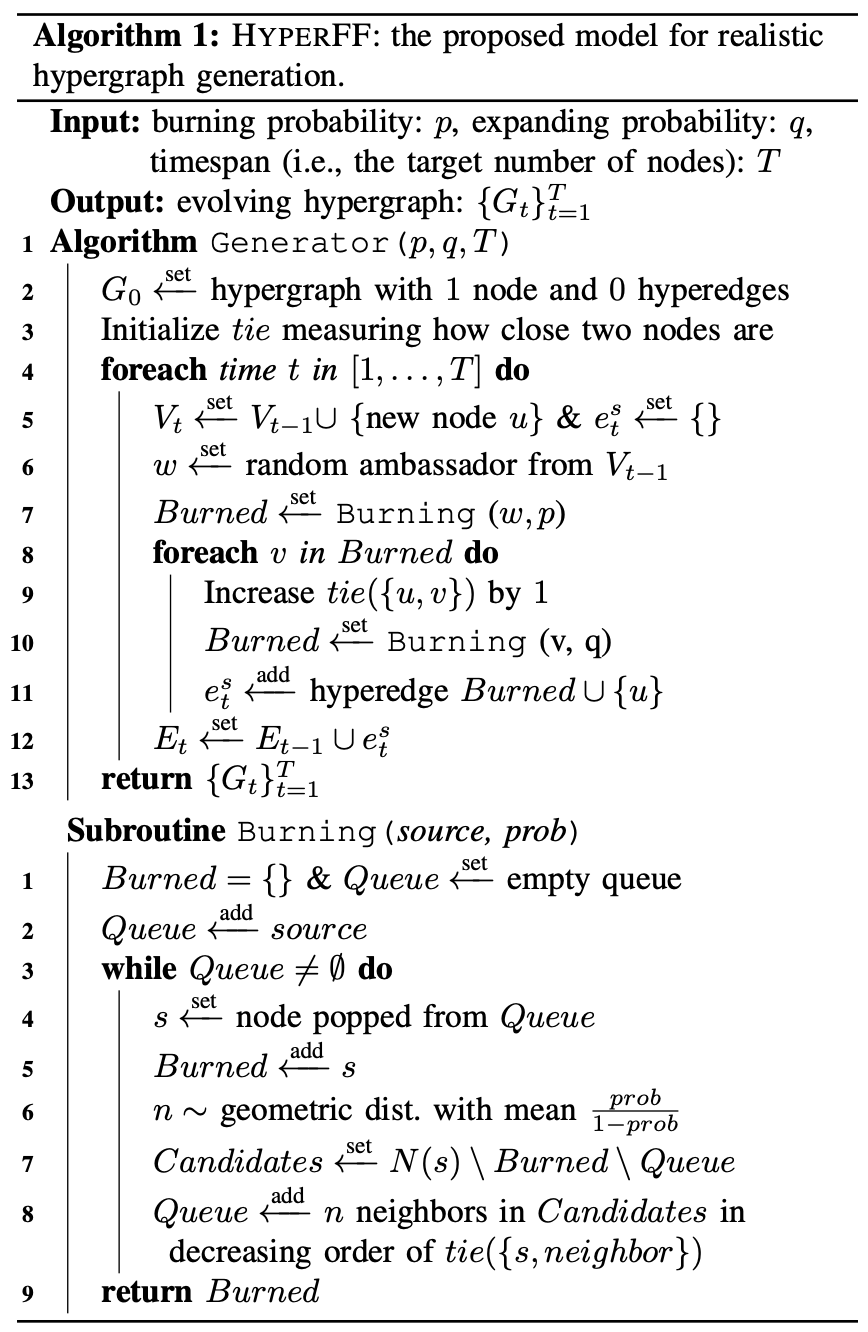
HyperFF(Hypergraph Forest Fire) , HyperPA 의 단점인 external factor 에 의존성이 강하다는 요소를 보완하기 위해 본 논문이 제안되었습니다. 이전 HyperPA 에서는 generation 시, 새로운 노드가 특정 그룹의 degree에 의존적이였었으나, 본 논문에서는 자생적으로 burning and expanding 하는 과정을 진행함으로써, 그 의존도를 낮춘거죠.

이전 논문 HyperPA와 다른점 두가지를 키워드로 설명해보자면 1. Plus take into dynamic patterns 2. self-contained for diminishing of oracles function. 이라고 할 수 있겠습니다.

Preliminary

[Goodness of Fit. , For evaluation empricial dataset to network science manner]

It is difficult to argue that an empirical dataset genuinely follows a target probability distribution, since other statistical models unexamined yet may describe the dataset with a better fit. Thus, it is more sound to rely on comparative tests which compare the goodness of fit of candidate distributions . We especially utilize the log likelihood-ratio test  to this end. When a dataset D with two candidate distributions A and B is given, the test computes $$log(L_{A}(D) / L_{B}(D)) , where LA(D) stands for the likelihood of the dataset D with respect to the candidate distribution A. Positive ratios imply the distribution A is a better description available for the dataset between the two distributions, and negative ratios imply the opposite.

Summary

서두에 설명드린바와 같이 이전 논문인 HyperPA에는 적용하지않은 dynamic pattern cretia도 포함하여 좀 더 엄밀한 hypergraph generator model 을 이야기합니다. 추가된 요소들은 다음과 같습니다.

1. (T1) 시간의 흐름에 따라 hyperedge overlapping 빈도수가 얼마나 감소하는지, 즉 교집합이 얼마나 줄어드는지를 측정합니다.
2. (T2) 시간의 흐름에 따라 node 대비 hyperedge가 얼마나 증가하는지를 측정합니다. densification 과 같은 요소를 예로 들 수 있습니다.
3. (T3) 시간의 흐름에 따라 노드들의 거리가 얼마나 감소하는지를 측정합니다. 예를 들면, shrinking diameter 과 같은 요소를 예로 들 수 있습니다.

이렇게 새로이 포함된 dynamic pattern 을 포함한채 structural , dynamic pattern creita 를 통해 generator performance 를 측정합니다.

이전 연구(HyperPA)에서는 New hyperedge 를 generation 할 때, 기존 hyperedge distribution 을 참고해서 진행했습니다. 그렇기에, 그 기준이 randomly selection 된 hyperedge 에 많이 의존적이다 라는 한계점이 존재했습니다. 그 한계점을 극복하기 위해 본 논문에서는 bruning 과 그 결과를 바탕으로 similarity 를 측정하여 expand 하는 방식을 제안합니다.

Insight

experiment 를 보시면 유독 Preliminary 에서 언급한 fitted line 이 많이 등장합니다. 해당 distribution 이 얼마나 타당한지를 fitted line 을 통해 간접적으로 확인할 수 있기에 generator 모델의 우수성을 검증하는 용도로 많이 활용합니다.

네트워크 견고성 측면으로 접근해보면 재밌는 인사이트가 많이 나올거라 생각됩니다. 예를 들어, 통신망 같은 경우 문제가 발생하고 난 후에 대책을 세워 액션을 진행하는 사후 대응이 아닌 사전에 문제가 될만한 요소를 파악해서 미리 방지를 하는 사전 대응이 중요할텐데요.

과연 사후에 무엇이 등장할지에 대해서는 너무나도 랜덤성이 강합니다. 그러기에 최대한 그 불확실성을 줄이는 방식을 채택하게 되는데요. 그 불확실성을 줄이기 위해 먼저 네트워크에서 어느 요소가 가장 중요하며, 취약성이 어느정도인지 관리를 해야합니다. 그 관리를 하기 위해서는 시뮬레이션이 필요하죠. 이때, 그 시뮬레이션 과정에서 자주 활용될 수 있는 방식이 본 논문의 아이디어라 생각합니다. pair-to-pair 그래프를 넘어 group interaction 측면에서 접근하기에 그 인사이트가 더하지 않을까 싶네요.

Graph Machine Learning Explainability with PyG

[https://medium.com/@pytorch_geometric/graph-machine-learning-explainability-with-pyg-ff13cffc23c2]

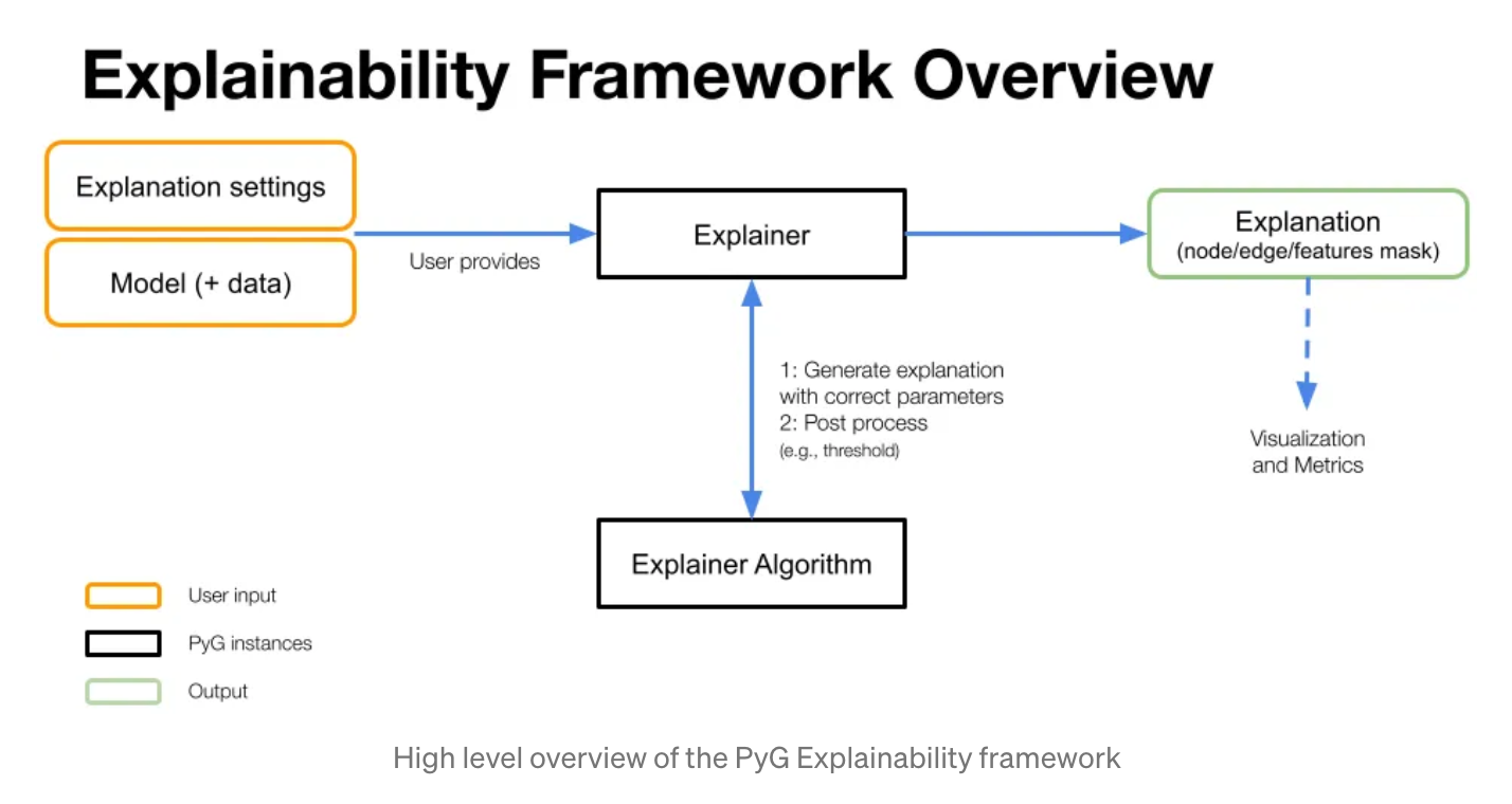
구현과 논문 트렌드 팔로우업 2가지 모든 요소를 고려하기 위해 저는 오마카세 이외에도 미디엄을 통해 PyG 에서 제공하는 Official tutorial을 reproduce 하는 시간을 주기적으로 가집니다. 그 중 이번에 소개시켜드린 포스팅은 XAI 관련해서 잘 설명되어있는 posting 입니다. GNN을 활용하며 성능이 왜 좋았는지 그리고 어떤 node,edge feature 덕분에 성능이 좋아졌는지에 대한 interpertation issue 가 있으셨던 분들에게 좋을 게시물입니다.